cycloid | Conversation of Momentum

Alan asked me an interesting question about a proton moving in a magnetic field. I hope he will forgive me for paraphrasing:

Consider a charged particle moving parallel to the ground in a uniform gravitational field. The gravitational force is normal to the ground. The charge immediately enters a region of uniform magnetic field orientated parallel to the ground, perpendicular to both the gravitational field and the charge’s initial velocity vector.

Provided the charge and the magnetic field have the correct sign, the Lorentz force will steer the charge up through the gravitational field. The charge will move in a semicircle, and leave the magnetic field, but at a higher point than that at which it entered.

In this way, the charge appears to have gained gravitational potential energy from nowhere. Has the conservation of energy been violated?

In the preamble above, I made an unproven assertion. I claimed that, simultaneously, there is a non-zero gravitational field and the charge moves in a semicircle. It is true that a charge moving in a plane normal to a uniform magnetic field will adopt a circular path. How do I know this is true in the presence of an additional gravitational field?

So rich and interesting is this simple physical problem that it warrants some discussion. In this relatively lengthy post, we will look in detail at the trajectories an electric charge may assume in uniform crossed $\bold{B}$ and $\bold{g}$ fields. We will first solve the equations of motion that describe the evolution of the charge’s spatial coordinates with time. Then we will explore the variety of trajectories available.

The quality of the animations has suffered a little in their previews, so please click on them to see them in their full glory in a new tab. All hail GeoGebra!

The particle has mass $m$ and charge $q$ .

Let the gravitational field $g$ be parallel to the $z$ axis. Let the magnetic field $B$ be parallel to the $x$ axis.

The particle starts at the origin:

$\bold{r}(0)= \bold{0}$

The charge enters the magnetic field horizontally, so at time $t=0$ its velocity is

$\bold{v}(0) = v_0\,\bold{j}$

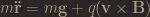
that is, parallel to the $y$ axis. In vector form, the equation of motion reads

$m\bold{\ddot{r}}=m\bold{g}+q(\bold{v}\times\bold{B})$

which in column vector notation is

$m\begin{pmatrix}\ddot{x}\\\ddot{y}\\\ddot{z}\end{pmatrix} = m\begin{pmatrix}0\\{0}\\-g \end{pmatrix} + q \begin{pmatrix} \dot{x}\\\dot{y}\\\dot{z} \end{pmatrix}\times\begin{pmatrix} 0\\ B\\ 0 \end{pmatrix}$

This gives the system of three differential equations

$m\ddot{x}=0$

$m\ddot{y} = qB\dot{z}$

$m\ddot{z} = -mg - qB\dot{y}$

The first equation is the simplest to solve. The particle does not accelerate in the $x$ direction, because both the gravitational and Lorentz forces act in the $yz$ plane.

This means the velocity in the $x$ direction will not vary with time. Making the $x$ velocity non-zero will not add any interesting new physics, so we will take it to be zero. This means

$x(t) = 0\ \forall\ t$

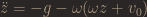
The second and third differential equations are coupled – each contains derivatives of both $y$ and $z$ . We will eliminate this dependence by integrating the second equation to give an expression for $\dot{y}$ in terms of $z$ . We will then substitute this expression into the third equation. This will yield a differential equation involving $z$ and its own derivatives only.

The second equation reads

$m\ddot{y}=qB\dot{z}$

With inexplicable foresight we will introduce the quantity

$\displaystyle \omega=\frac{qB}{m}$

$\displaystyle \frac{d\dot{y}}{dt} = \omega \frac{dz}{dt}$

Integrating up,

$\displaystyle \int_{v_0}^{\dot{y}}\frac{d\dot{y}}{dt}dt = \omega\int_0^z \frac{dz}{dt}dt$

$\dot{y}= \omega z+v_0$

We now substitute this expression into the third equation:

$m\ddot{z} = -mg - qB\dot{y}$

$m\ddot{z} = -mg - qB(\omega z+v_0)$

$\ddot{z} = -g - \omega(\omega z+v_0)$

$\ddot{z} + {\omega}^2 z=-(g+\omega v_0)$

The most general solution to this equation is

$\displaystyle z(t)=P \cos\omega t + Q \sin\omega t - \frac{g+\omega v_0}{{\omega}^2}$

where $P$ and $Q$ are constants. The constant term on the right is the so-called particular integral, an educated guess. The trigonometric terms form the complementary function, which can be added on to the solution ‘for free’ since they satisfy $\ddot{z} + {\omega}^2 z = 0$ .

That $z(0)=0$ sets

$\displaystyle P = \frac{g+\omega v_0}{{\omega}^2}$

and $\dot{z}(0) = 0$ means

$Q = 0$

Hence

$\displaystyle z(t)=\Big(\frac{g+\omega v_0}{{\omega}^2}\Big)(\cos\omega t - 1)$

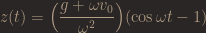
We then substitute this into our equation for $\dot{y}$ ,

$\dot{y}=\omega z + v_0$

$\displaystyle \dot{y}=\omega\Big(\frac{g+\omega v_0}{{\omega}^2}\Big)(\cos\omega t - 1) + v_0$

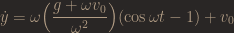
and integrate, imposing initial conditions:

$\displaystyle y(t)=\Big(\frac{g+\omega v_0}{\omega}\Big)(\sin\omega t - t) + v_0 t$

So we have obtained the charge’s trajectory. The position vector of the charge as a function of time is

$\bold{r}(t) = \begin{pmatrix}0\\\big(\frac{g+\omega v_0}{\omega}\big)(\sin\omega t - t) + v_0 t\\\big(\frac{g+\omega v_0}{{\omega}^2}\big)(\cos\omega t - 1)\end{pmatrix}$

Let’s now explore the family of trajectories by varying the featured parameters. We’ll first consider the most interesting effect, that of changing the initial velocity $v_0$ .

Suppose the charge is released from rest, so $v_0=0$ . In this case, the trajectory is described as a cycloid. A cycloid is the curve traced out by a point fixed on the circumference of a rolling circle. The animation below shows the motion of the charge for $qB<0$ in the $yz$ plane and the force acting on it.

There are several comments to be made.

This first and most obvious: this is a beautiful result.

The second: the charge will not fall. As the charge begins to gain velocity downward, it starts to experience a Lorentz force in the positive $y$ direction. As soon as the charge has a non-zero rightward velocity, there is a component of the Lorentz force acting upwards, decreasing the rate at which the charge is falling. Eventually, the charge has been steered round to such an extent that it is travelling horizontally. At this point, the Lorentz force acts exclusively in the positive $z$ direction, dragging the charge upwards. The charge ultimately comes to rest at the same height as where it started. The pattern repeats.

The form of this trajectory is identical for all values of $g, m, q$ and $B$ ; only its scale varies. Increasing either $g$ or $m$ increases its size. Increasing the magnitude of $B$ or $q$ decreases it. Changing the sign of $qB$ causes the charge to move in the negative $y$ direction instead.

The rate at which the charge completes a ‘cycle’ is dictated by the angular frequency $\omega$ , which we defined as

$\displaystyle \omega=\frac{qB}{m}$

This result is quite intuitive. The greater the magnitude of $qB$ , the greater the strength of the coupling between the charge and the magnetic field. Hence the rate at which the particle’s path deviates from a straight vertical line is increased. The greater the value of $m$ , the more the charge resists the effect of the magnetic field and the slower is deviation from the vertical line.

Let us look at the more general case.

We’ll gradually increase $v_0$ from zero to a positive value:

The trajectory is a called a trochoid, of the the cycloid is a special case. Note the positions at which the charge meets the $y$ axis is invariant.

The trajectory passes through several interesting states as $v_0$ is increased.

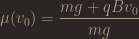
For small $v_0$ , the cusps of the cycloid soften into smoothed hills. The name for this particular curve is a curtate trochoid.

As the initial velocity is increased further, you may notice that there exists a value of $v_0$ at which the trajectory is a straight line. From the expression for $\bold{r}$ , this occurs when

$g+\omega v_0=0$

When this equation is satisfied, the force on the charge vanishes.

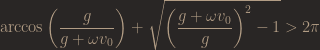
Next, the trajectory forms another curtate trochoid, eventually becoming another cycloid above the $y$ axis. This cycloid has a $\frac{1}{2}\pi$ phase shift relative to that for which $v_0=0$ .

This occurs when there exist solutions to the equation

$\dot{y}=0$

which can be shown to occur when

$\displaystyle \frac{g}{g+\omega v_0}\le 1$

Above this velocity, the charge starts to draw loops. Increasing the launch velocity distends the loops. This looping pattern is called a prolate trochoid.

Increasing the initial velocity $v_0$ further yet causes the charge to take a path which allows it to escape the magnetic field, assuming $B=0$ for $y<0$ . Some algebra shows that this happens if

$\displaystyle \arccos\bigg(\frac{g}{g+\omega v_0}\bigg)+\sqrt{\bigg(\frac{g+\omega v_0}{g}\bigg)^2-1}>2\pi$

This equation cannot, as far as I know, be solved analytically. A numerical solution is given below. It is quite interesting that this fraction

$\displaystyle \frac{g+\omega v_0}{g}=\frac{mg+qBv_0}{mg}$

has appeared again. In fact, we can predict which trochoid the charge’s motion will assume based purely on the value of this fraction.

We’ll define the quantity $\mu$ as

$\displaystyle \mu(v_0)=\frac{mg+qBv_0}{mg}$

Combing all of the previously established results, we know that for

$\mu=1$ , the trajectory is a cycloid below the $y$ axis
$1>\mu>0$ , the trajectory is a curtate trochoid below the $y$ axis
$\mu=0$ , the trajectory is a straight line along the $y$ axis
$0>\mu>-1$ , the trajectory is a curtate trochoid above the $y$ axis
$\mu=-1$ , the trajectory is a cycloid above the $y$ axis
$-1<\mu<-4.6$ , the trajectory is a prolate trochoid in the first quadrant
$\mu<-4.6$ , the particle can escape into the region $y<0$

where the number $-4.6$ is computed numerically. It is remarkable that the value of this simple linear equation in the initial velocity $v_0$ tells us which member of the trochoid family the trajectory will assume. Here is another animation showing the trajectory evolution along with the value of $\mu$ in the top right corner.

The conditions on $\mu$ can be easily inverted to give conditions for $v_0$ in relation to $g, B$ and $m$ instead.

As a sanity check, we can also watch how the particle’s trajectory changes as the gravitational field $\bold{g}$ is switched off:

The trajectory tends to a circle, as we expect. For small $g$ , the charge moves in an almost circular path which drifts slowly to the right.

So, applying a gravitational field downwards causes the charge to migrate sideways!

On a final note, the dependence of the force on the charge with time goes like

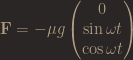
$\bold{F}=-\mu g \begin{pmatrix}0\\\sin\omega t\\\cos\omega t\end{pmatrix}$

for $g\ne 0$ . Every trajectory above is produced by a force vector which rotates at a fixed frequency, like a phasor.

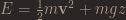
It can be shown from the expression for $\bold{r}(t)$ that the total energy of the charge,

$E=\frac{1}{2}m\bold{v}^2+mgz$

is equal to

$E=\frac{1}{2}mv_0^2$

that is, mechanical energy is conserved. This shows that the particle cannot gain energy for free.

It’s likely that I’ve only scratched the surface of the physics encoded in these equations. In my next post, I’ll be looking more at the mechanics of a charge in a magnetic field.

Conversation of Momentum

No, That's Not a Typo

Tag Archives: cycloid

Crossed B and g fields

Share this: